归档
一些思考后给出答案,但是不成体系的问题。
概率空间定义要用三个要素
概率空间定义,样本空间、事件空间、概率测度
我们直觉上、习惯上是将概率定义在样本空间上,然而实际上严格定义是在事件空间上,事件空间是sigma代数,
这是为了解释当样本空间有不可数集的时候,如何定义概率的问题。
泛函“只”有一阶导
泛函是函数向实数域的映射。
泛函取极值的必要条件是euler-lagrange方程成立。
我们看到的euler-lagrange方程是依赖于路径、路径导数和自变量的微分方程。
广义的euler-lagrange方程依赖路径的更高阶导数。
最速降线没有用广义euler-lagrange方程只是采用euler-lagrange方程的标准形就能解出来路径方程,并且和事实相符。
动态规划是强化学习
动态规划是有模型强化学习。有模型强化学习不需要通过数据进行训练。动态规划的不同状态是指具有不一样的参数的同一个优化问题。
比如背包问题,背包容量不一样,物品数量不一样,就是一个状态。
形式化成一个优化问题后,发现可以通过max,min或者分段函数这样的非线性操作进行状态转化,转移函数就对应强化学习里的模型。
动态规划能解的问题很有限,不能有后效性,且初始子问题足够简单,才能求解。找转移函数的过程比较困难,需要积累。
背包dp,序列dp,树状dp,DAG-dp等。
Caffe代码结构
caffe组织推理的过程分为四层结构:syncedmem -> blob -> layer -> net
syncedmem是最底层的线性数据结构,用来维护cpu和gpu的存储同步。blob是更高一层的抽象,维护张量的形状和数据,是所有张量操作的基本类型。layer是构成神经网络的基本单元,net就是最终的推理结构。
Caffe除了完成推理,还要执行训练,对异构设备的适应,以及对单独CPU执行的支持,因此Caffe对于内存进行syncedmem这一层的封装。我们只需要在前向推理时实现多流并发,syncedmem这一层封装可以不需要,可以在blob内部完成内存和显存的数据转化和分配。
im2col对卷积的实现
二维卷积的朴素实现包括7个循环:batch_size,输出通道数量、输入通道数量、卷积核高、卷积核宽、沿宽方向滑动距离、延高方向滑动距离。以此类推,三维卷积9个循环。
这么多循环放在CUDA中,不利于优化,且缓存不命中,频繁访存执行效率低。考虑到卷积核和输入张量对应点的相乘,与向量点乘的运算过程是一样的,而矩阵乘法是向量点乘的堆叠,因此可以设计一种先将输入转化成矩阵,然后执行矩阵的相乘加速卷积速度的方法。
方法改变,结果不改变,应保证转化+矩阵相乘与朴素实现的输出结果一样。
朴素卷积输出张量$O$的维度是
[batch_size, conv_out_channels, spatial_output_shape_h, spatial_output_shape_w],
卷积层保存的权重$W$维度是
[conv_out_channels, conv_in_channels, kernel_h, kernel_w]。
卷积核的维度就是
[conv_in_channels, kernel_h, kernel_w]
设$O = W * D$,$D$是输入张量转化而来形成的矩阵。考虑到张量在内存和显存中均是一维存储,可以将$W$视作行数为conv_out_channels,列数为conv_in_channels * kernel_h * kernel_w的矩阵,$O$视作行数为batch_size * conv_out_channels,列数为spatial_h * spatial_w的矩阵。
转化得来的矩阵$D$的行数需要是$W$的列数,列数是$O$的列数,才能满足$O = W * D$的表达式。同时左矩阵的行向量与右矩阵的列向量点乘需要等价于卷积核和张量对应区域的相乘。
考虑batch_size中的输入张量独立,因此可将$O$划分成batch_size个张量,$D$的行数为conv_in_channels * kernel_h * kernel_w,列数为spatial_h * spatial_w,从而首先确定维度。其次,根据$O$中列号对应的输出张量空间位置,计算在原始输入张量的空间位置中的哪些元素与卷积核相乘,在输入张量中按行展开这些元素,按卷积核通道序号次序放入列号对应的列向量。
计算方式如下代码所示。
1 | /* compute the output_spatial_shape */ |
从输出张量反推输入张量位置是计算的关键步骤,对应即是h_offset、w_offset以及data_im_ptr的计算过程。卷积的整体前向传播过程即分为两步。
1 | void ConvolutionLayer::Forward(const std::vector<Blob*>& bottom, const std::vector<Blob*>& top, cudaStream_t stream) { |
C语言宏的替换
第一种,被替换对象是被标点或空格分割开的“独立字符串”,用#表示。
第二种,被替换对象被一个独立字符串真包含,用##表示,当被替换对象位于独立字符串开头,则在被替换对象的结尾加##表征;当被替换对象位于独立字符串结尾,则在被替换对象的头部加##表征;当被替换对象位于独立字符串中间,则在被替换对象的开头和结尾都加##表征。
例子:
1 |
|
C语言静态库
静态库方便移植,速度快,但是体积大,编译慢,这个都知道。除此之外,静态库中的static变量不会被事先声明,如果在头文件定义static变量,可能有重复定义的风险。
怎么解决呢?制作一个只有可能被应用程序引用的头文件,在其中定义需要预先定义的static变量。
例子:不同layer初始化注册map表。
1 | /* register_layer.h */ |
C++内存分配
C++为了避免手动free或者delete的问题引入std::shared_ptr<>,即智能指针。智能指针调用对象方法时和一般指针一样,变成一般指针时用.get()方法.
当具有独显时:
C++仅有分配内存的能力,显存的分配用CUDA接口;
gpu计算单元不能访问内存,cpu也不能访问显存,
显存和内存可以互通,但是显存分配不提供智能指针,仅提供原始类型的指针。
core dump
一般逻辑问题查找日志基本可以解决。Core Dump没有日志报错信息,或者日志容易出问题。这时需要用调试工具。
使用gdb+cmake编译时,添加-g编译选项,如下段代码。用ulimit -c nolimited取消core dump文件的大小限制。更改/proc/sys/kernel/core_pattern的core dump文件输出位置和命名,然后用gdb <程序名> <修改后的coredump文件名> 进入gdb调试。在gdb中用bt查找调用栈,一般能定位内存出问题的位置。
1 | # CMakeLists.txt |
工厂模式的好处
神经网络前向推理初始化的时候,每个层需要根据InferParameter中定义的layer编号类型定义并创建。不同类型的layer对应抽象layer的不同子类实现,如果没有工厂模式的话,需要在初始化layer的时候,根据layer的类型一一对应写出其构造函数,当类型很多时,这一步很繁琐。
用工厂模式,就是初始化的时候很简单,一行代码,工厂模式自己找到对应的构造函数,如下所示。
1 | for (int layer_id = 0; layer_id < para.layer_size(); layer_id++) { |
这个函数对应实现如下,在一个全局维护的map中,根据layer类型查找对应的初始化函数。
1 |
|
除此之外,工厂模式中每个layer都有自己的特殊SetUp函数,如下面第5行代码所示,也不用根据type类型再写额外的判断逻辑。(也是C++重载的好处?指向基类的指针调用不同子类的重载函数?)总之,工厂模式,就是为了在使用“工厂”的产品时,不用加一堆分支判断逻辑。(其实就两字:方便!)
1 | for (int layer_id = 0; layer_id < para.layer_size(); layer_id++) { |
那么工厂模式如何实现的呢?第一,多种layer实现时需要采用继承的方法;第二是维护一个全局的初始化函数表,这样在初始化时查找这个表就可以避免写判断逻辑,这个初始化表可以在类实现中直接注册。
1 |
|
比如这段代码中,LayerRegisterer的初始化调用了一个static方法实现creator的注册,这两个宏实现了这个类的初始化,所以我们看到只需要一行代码就可以实现不同layer子类的注册。
CUBLAS加速矩阵乘法的一个小问题
矩阵、张量在内存和显存中均以一维方式存储。
在CUBLAS中,GPU的计算单元读取矩阵的方式是按列读取和放回显存。我们习惯内存、显存以及cpu以行优先的方式读取。CUBLAS提供的API就不会很习惯,因此做一个封装使得外界使用时仍然按照习惯写法,但是内部仍用CUBLAS加速。
采用的方式调用CUBLAS的API的时候将A和B顺序反过来。这是因为CUBLAS读取的是转置,若$C=AB$,则$C^T=B^T \times A^T$,而$C^T$在GPU计算单元写回的时候是列优先顺序,则按照行优先读取的时候就是$C$,所以在封装内部调用CUBLAS的API的时候将A和B顺序反过来即可。
代码如下
1 | void acc_gemm( |
caffe中blob的初始化方式
caffe,又称blobflow。
caffe是用来实现各种各样神经网络前向推理,和反向传播的框架。神经网络由各种layer组合构成,caffe自身提供了卷积、全连接等层的实现。
由于layer的是存储密集、计算密集型的任务,且适用并行加速,因此涉及到cpu、内存、显存和gpu之间的切换。另外layer的输入、输出,自身权重都是高维张量构成,而数据在内存和显存的存储为一维结构,因此维度、数据的长度、显存和内存的同步这三个因素需要被考虑。
caffe用blob表征权重、输入和输出等张量。blob逻辑上描述了张量维度、展平后的数据长度。也描述了blob数据对应的导数数据,如果只做前向传播的话这部分数据是用不到的。blob的默认初始化不分配内存和显存,张量维度和展平后数据长度默认为0。blob的显示初始化对应分别对应权重张量和输入输出张量的存储分配。
权重的张量维度、展平后的数据长度在模型文件中被定义,因此caffe定义第一种初始化和保存方式:
1 | void FromProto(const BlobProto& proto, bool reshape = true); |
针对前向推理以及反向传播的中间计算结果、即输入张量和输出张量,caffe定义了第二种初始化方式:这种初始化方式调用了Reshape函数,Reshape当中会为数据分配内存和显存。
1 | explicit Blob(const vector<int>& shape); |
和第一种方式的区别是这种方式只定义张量维度,不对数据的值做要求,采用这种接口的原因是中间张量的数据并不是我们需要保存的权重,只是需要在显存中开辟张量存储的空间。
由于前向推理时大部分Layer的设计中,(1)输出张量的维度依赖输入张量的维度,(2)并且上一层的输出张量一般是下一层的输出张量,因此Layer在初始化时,一般要求输入张量bottom的维度确定并完成内存显存分配,在调用SetUp函数时再确定输出张量top的维度并完成存储空间分配。多个Layer构成的推理流在初始化时,也要遵循这一设定。
1 | void SetUp(const std::vector<Blob*>& bottom, const std::vector<Blob*>& top) { |
CMake编译系统
环境gcc7.5.0,ubuntu18.04,cmake3.25.0。
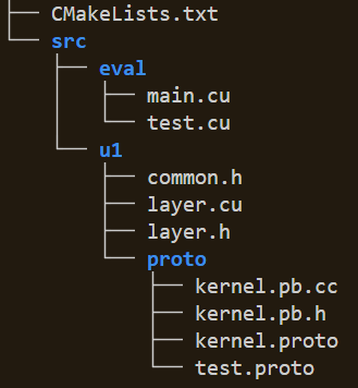
整体结构如上图所示,u1文件夹里是写好的算法代码,eval文件夹里是基于算法编写的应用程序,包括测试、实验对比、调用程序等。
因为用到protobuf,所以需要先对proto文件处理生成对应*.pb.cc和*.pb.h文件,这两个文件内容比较多,先把其编译成独立的库,而不是直接和u1里的代码混编,第二步编译u1,最后编译eval里的应用程序。
有几个点注意:第一头文件和执行文件放在一起,所以不设置单独include文件夹,第二cmake版本小于3.10需要手动引入cuda库。
因此CMakeLists.txt的书写方法如下:
1 | cmake_minimum_required(VERSION 3.10) |
先声明项目需要用到语言,因为是GCC7.5.0,默认C++11标准。
1 | include_directories("${PROJECT_SOURCE_DIR}/src") |
声明头文件额外引入路径和需要编译的库目录
1 | find_package(gflags REQUIRED) |
声明需要用到的包,glog,gflags和protobuf是我做C++开发比较喜欢用的库。
1 | # protoc -I=. --cpp_out=. kernel.proto |
生成kernel.proto对应的c++ API文件
1 | add_library( |
然后分别生成库文件,包括定义接口的库以及算法库。
1 | function(add_executable_app app_name app_path) |
最后生成应用程序、测试程序和用来比较的实验数据。
梯度下降
现实世界中的诸多任务可以被抽象成一个接收一定形式的输入,并产生某种类型输出的函数。然而对于现实世界中的大部分任务,其函数关系复杂且普遍具有非线性关系,无法轻松找到这样的函数。
神经网络算法的目的就是通过神经网络结构表征任务的非线性特征,并通过已有数据集产生神经网络参数,从而拟合现实世界任务对应的函数,这个函数可以被表示为
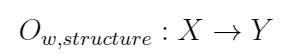
其中$structure$表示神经网络的结构,该结构是神经网络拟合现实任务非线性特征的关键,通常情况下是先验的,需要研究人员精心设计得到,比如transformer和conv结构。
$X,Y$表示数据集中的输入和输出,参数$w$是神经网络参数。在模型获取阶段(训练),我们能够同时拿到数据集的输入和输出$X,Y$,并希望得到神经网络参数$w$;在模型应用阶段(推理),我们只拿到数据集中的$X$(输入数据),希望得到和真实世界任务尽可能相近的结果$Y$。
在模型推理阶段中,由于我们已经得到了神经网络参数$w$,获得结果的过程是一个前向计算的过程,按步骤执行即可。
而在模型训练阶段,神经网络参数$w$是未知的,而函数$O(X)$的输出是已知的,由于神经网络参数$w$通常是高维向量,数据集$X,Y$同样具有一定规模,这相当于是在近似求解一个高维方程,这个问题通常是难解的,因此需要梯度下降,也就是反向传播过程。
将近似求解高维方程的问题转化为最小化loss函数的问题,令
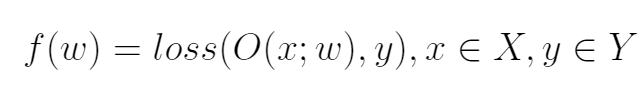
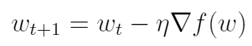
在反向传播过程当中,由于数据集中的输入和输出都是已知的,即让该函数最小即可,根据优化理论,按照下式不断迭代,直到loss函数的变化小于某阈值即可。
这里讨论一些梯度下降方法中确保准确率的一些难点。
关于数据集:由于数据集是通过实践获得的,只有统计意义上的理论保证。所以在每一轮迭代过程中如何选取数据集,如何保证数据集之间的偏差在一定范围内?
关于神经网络结构:由于神经网络的层状结构,存在梯度消失,梯度精度等问题
Lipschitz Continuity
In mathematical analysis, Lipschitz continuity, named after German mathematician Rudolf Lipschitz, is a strong form of uniform continuity for functions. Intuitively, a Lipschitz continuous function is limited in how fast it can change: there exists a real number such that, for every pair of points on the graph of this function, the absolute value of the slope of the line connecting them is not greater than this real number; the smallest such bound is called the Lipschitz constant of the function (or modulus of uniform continuity). For instance, every function that has bounded first derivatives is Lipschitz continuous.
We have following chain of strict inclusions for functions
over a closed and bounded non-trivial interval of the real line (So strong!)Continuously Differentiable $\subset$ Lipschitz Continuous
$\subset$ $\alpha-$ Holder Continuous $\subset$ Uniformly Continuous = Continuous
Lipschitz Continuity Defintion:
Given two metric spaces $(X, dX)$ and $(Y, dY)$, where $dX$ denotes the metric on the set $X$ and $dY$ is the metric on set $Y$, a function $f : X \rightarrow Y$ is called Lipschitz continuous if there exists a real constant $K \geqslant 0$ such that, for all $x_1$ and $x_2$ in $X$,
Metric Space
In mathematics, a metric space is a nonempty set together with a metric on the set. The metric is a function that defines a concept of distance between any two members of the set, which are usually called points.
The metric satisfies a few simple properties:
the distance from $A$ to $B$ is zero if and only if A and B are the same point.
the distance between two points are positive.
the distance from $A$ to $B$ is the same as the distance from $B$ to $A$, and
the distance from $A$ to $B$ is less than or equal to the distance from A to B via any third point C.
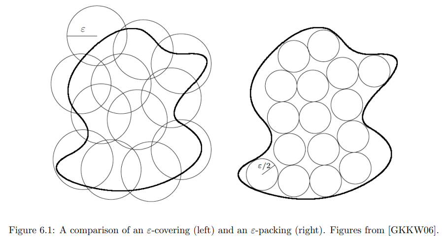
Covering Number and Packing Number
In mathematics, a covering number is the number of spherical balls of a given size needed to completely cover a given space, with possible overlaps.
Two related concepts are the packing number, the number of disjoint balls that fit in a space, and the metric entropy, the number of points that fit in a space when constrained to lie at some fixed minimum distance apart.
Let $(Z, d)$ be a metric space, let $K$ be a subset of $Z$, and let r be a positive real number. Let $B_r(x)$ denote the ball of radius $r$ centered at $x$. A subset $C$ of $Z$ is an $r-external$ covering of $K$ if:
In other words, for every $y \in K$ there exists $x \in C$ such that $d(x,y) \leqslant r$.
If furthermore $C$ is a subset of $K$, then it is an r-internal covering.
The external covering number of $K$, denoted $N_{r}^{\text{ext}}(K)$, is the minimum cardinality of any external covering of K. The internal covering number, denoted $N_{r}^{\text{int}}(K)$, is the minimum cardinality of any internal covering.
A subset $P$ of $K$ is a packing if $P \subseteq K$ and the set ${B_{r}(x)}_{x\in P}$ is pairwise disjoint. The packing number of $K$, denoted $N_{r}^{\text{pack}}(K)$, is the maximum cardinality of any packing of $K$.
A subset $S$ of $K$ is r-separated if each pair of points $x$ and $y$ in $S$ satisfies $d(x, y) \geqslant r$. The metric entropy of $K$, denoted $N_{r}^{\text{met}}(K)$, is the maximum cardinality of any r-separated subset of $K$.
Covering number and packing number will be written as $N(Z, d, r), M(Z, d, r), $ respectively.
Metric entropy also equals to $log N(Z, d, r)$.